Neural Network from Scratch
Table of Content
3. Combination of Functions
4. Forward Pass 5. How to update weights? 6. Chain Rule 7. Implementing the Backward pass 8. Understanding the DOT PRODUCT
9. Conclusion
Overview
In our previous blog, "Understanding Tensors in
PyTorch" we explored the basics of tensors, which are fundamental and
powerful data structures in neural networks. Those sections laid a strong
foundation
for learning how to build a neural network from scratch.
In this section, we will take a deeper dive into the building blocks
of
neural networks. We will start by understanding the dot product, a crucial
mathematical operation in neural networks. Then, we will walk through coding a
neural network from scratch, step by step.
We will cover the following key topics:
1. Basic Building Blocks: Understanding the essential components that make up a neural network.
2. Dot Product: Learning how the dot product works and why it is important in neural network computations.
3. Neural Network Coding: Implementing a simple neural network from scratch, including forward propagation, activation functions, and backpropagation for training.
By the end of this section, you will have a solid
understanding
of how neural networks operate at a fundamental level and be able to create your
own
basic neural network model from scratch.
Let's continue our journey into the fascinating world of neural networks and
unlock
the potential of deep learning!
Introduction
Neural networks are one of the most popular machine learning
algorithms. They have been successfully used in many areas like image
classification
and time series forecasting, making them valuable in both business and research.
Understanding how neural networks work is crucial because it helps diagnose
issues
and lays the groundwork for learning more advanced deep learning algorithms.
In this article, we will break down how a neural network works. We will go
through
the algorithm step-by-step and show you how to set up a simple neural network in
PyTorch.
Combination of Functions
Let's start with some basic concepts. Imagine two simple linear functions:
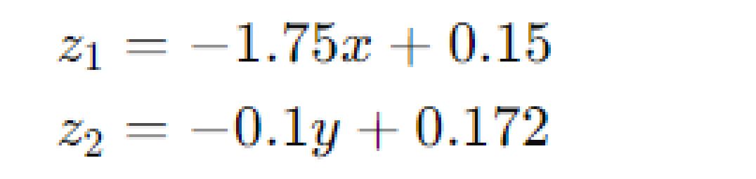
Here, the coefficients (-1.75, -0.1, 0.172, 0.15) are chosen just for illustration. Now, we define two new functions, a1 and a2, using a special function called the sigmoid function:
The sigmoid function, σ(x) creates an S-shaped curve and plays a key role in neural networks.
Next, we define another function that combines a1 and a2 linearly:
z3=0.25a1+0.5a2+0.2
Again, the coefficients (0.25, 0.5, 0.2) are arbitrarily chosen. By combining these functions, we create more complex functions capable of capturing intricate patterns. For example, the combined function z3 looks more complex than a1 or a2.
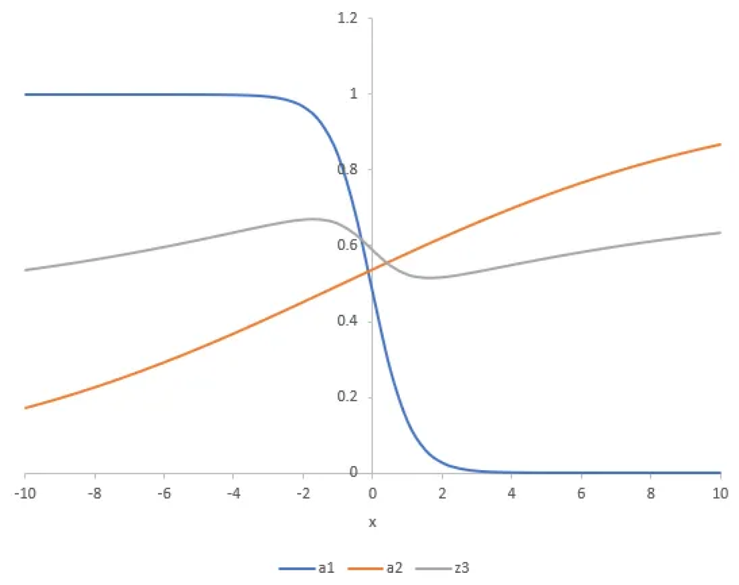
If we apply the sigmoid function to z3 and combine it with
another similar function, we can create even more complex patterns. By adjusting
the
coefficients, we can fit our final function to complex data sets. This is the
basic
idea behind neural networks: combining simpler
functions
to represent complicated variations in data.
Now, let's delve into the framework of a neural network and see how it all comes
together.
Forward Pass
Now, let's introduce the concept of a forward pass in a
neural
network. The forward pass is the process of moving input data through the
network to
get an output. This involves multiple layers, each performing specific
calculations
on the data and passing the results to the next layer.
Here is an example:
As shown in the diagram, we start with our training data X.
This
data is fed into the first layer of our neural network. Initially, this layer
uses
randomly assigned weights and biases. These weights and biases are the
parameters
that our model will learn and optimize during the training process.
The output from this layer is then passed through an activation function. The
activation function introduces non-linearity
into
the model, allowing it to learn and represent complex patterns in the data.
Common
activation functions include the sigmoid, ReLU, and tanh functions.
After applying the activation function, we get a set of predictions from the
neural
network. These predictions are then compared to the true values (the actual
labels
or outcomes we want to predict) to calculate the loss. The loss is a measure of
how
far off our predictions are from the true values. A common loss function for
classification tasks is cross-entropy loss, while mean squared error is often
used
for regression tasks.
The optimizer then comes into play. The optimizer uses the calculated loss to
adjust
the weights and biases in the neural network, with the goal of reducing the loss
in
future iterations. Popular optimization algorithms include gradient descent,
Adam,
and RMSprop. The optimizer updates the weights by computing the gradient of the
loss
function with respect to each weight and bias, and then making adjustments in
the
direction that minimizes the loss.
This process of passing data through the layers, applying activation functions,
calculating loss, and updating weights is known as the forward pass. It is
repeated
for many iterations, or epochs, allowing the neural network to learn and improve
its
performance over time.
By continually optimizing the weights and biases, the neural network becomes
better
at making accurate predictions. This iterative process of training helps the
model
generalize well to new, unseen data
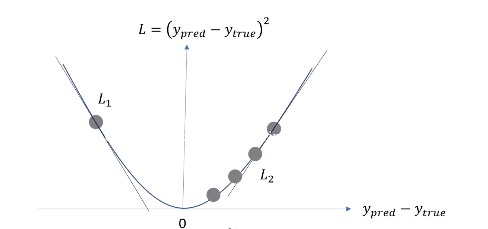
How to update weights?:
To understand how weights are updated in a neural network,
let's
revisit what we got from our forward pass. We spoke about the loss calculation
or
error, which measures the difference between our predicted values and true
values.
This difference is plotted along the X-axis, while the Y-axis corresponds to the
actual loss. Because we're squaring the differences, the loss function curve
takes
on a U-shape.
The objective of our optimizer is to minimize this loss. Ideally, the goal is to
bring this loss function value as close to zero as possible. In the real world,
the
loss function values won't be exactly zero, but we will aim for values close to
it,
like L1 or L2, as shown in the diagram. If we get a loss value of L1, we need to
increase the difference to reach the minimum value. Conversely, if we get a loss
value of L2, we need to decrease the difference.
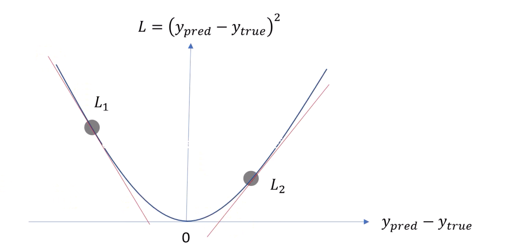
To achieve this, we need to delve into a bit of mathematics.
We
can place a tangent (shown as a red line) on the curve of the loss function.
This
tangent represents the gradient, which is the
derivative of the loss function. This process is called
gradient descent. We use these gradients to update the weights.
Regardless of whether we're at L1 or L2, the gradient will guide us in the right
direction to minimize the loss.
If you are far from the optimal minimum point, your gradient will be larger,
indicating a larger error. Larger errors result in larger absolute gradients.
This
is where the concept of "Learning Rate" into
play.
Let's consider the scenario where our error is at L1. If we do not have a
learning
rate, it is possible that we might overshoot the minimum point and jump to the
other
side, reaching L2, and then oscillate between L1 and L2. This means we might
never
reach the minimum. To handle this problem, we introduce something called the
learning rate.
Wnew = W - (dL/dw . LR)
The learning rate controls how much we adjust the weights
with
respect to the gradient. Instead of subtracting the entire gradient from the
current
weight, we multiply the gradient by the learning rate and then subtract this
product
from the weights. Typical learning rates are values like
0.01, 0.001, etc
Choosing the right learning rate is crucial. A learning rate that is too high
can
cause the model to converge too quickly to a suboptimal solution, or even
diverge,
while a learning rate that is too low can make the training process very
slow.
In summary, the process of updating weights involves:
1. Calculating the gradient of the loss function with respect to the weights.
2. Multiplying this gradient by the learning rate
3. Subtracting the result from the current weights to get the updated weights
This process ensures that we make small, controlled steps towards minimizing the loss, ultimately leading to a well-trained neural network.
Chain Rule
In the previous section, we discussed how gradients and learning
rates are used to update the weights in a neural network. Now, let's dive into the
chain
rule, a crucial concept for calculating gradients in neural networks, particularly
during the backward pass.
Imagine we have an input vector X, and this is passed through a function y=f(X).
This
function y is dependent on X. Then, we pass y through another function to get
z=g(y),
which makes z dependent on y. Our goal is to find the derivative of z with respect
to X,
denoted as dz/dx.
The chain rule helps us achieve this. According to the chain rule, to get dz/dx, we
need to first compute the derivative of y with respect to X, denoted as dy/dx.
Next, we
calculate the derivative of z with respect to y, denoted as dz/dy. Finally, we
multiply
these two derivatives to get dz/dx:
dz/dx=dz/dy . dy/dX
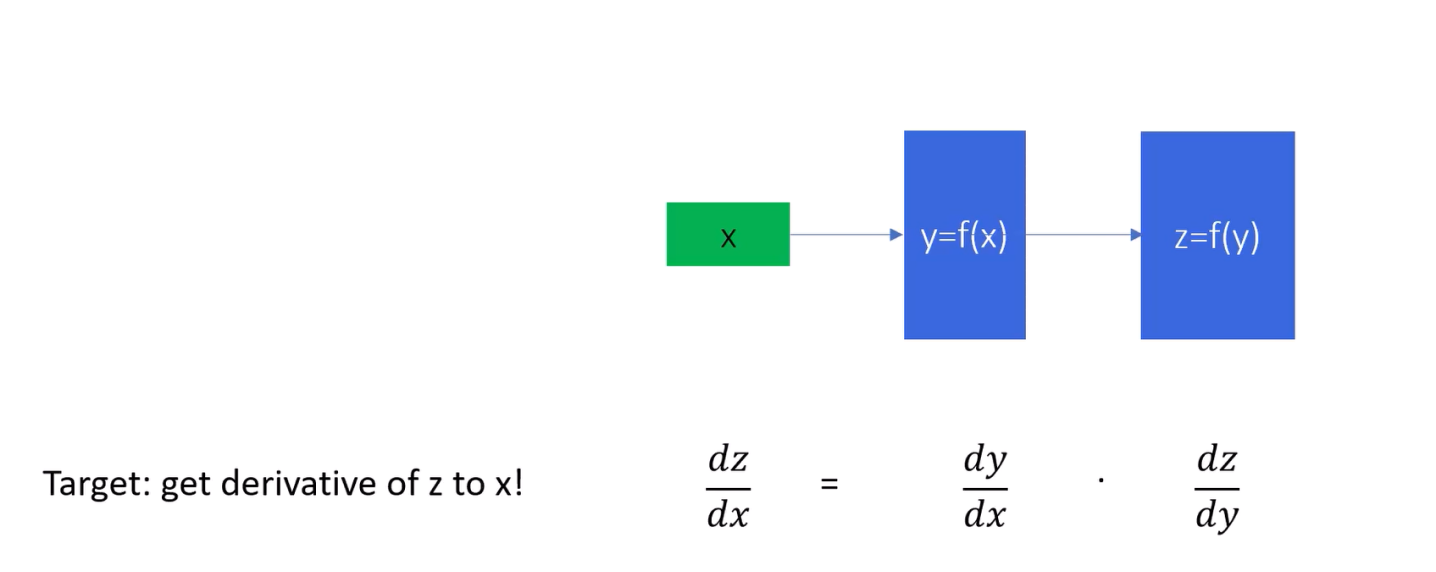
Let’s break this down with an example. Consider the above
diagram:
Here, X is our input vector, y is the output of the first function f(x), and z is
the
output of the second function f(y).
1. Calculate dy/dx: Suppose f(X) = X^2. The derivative of y with respect to X is dy/dx=2X.
2. Calculate dz/dy: Now, let’s say f(y)=sin(y). The derivative of z with respect to y is dz/dy=cos(y)
3. Apply the Chain Rule: To find dz/dx, we multiply these two derivatives:
dz/dx=cos(y)×2X
However, since y=X^2, we substitute y back in:
dz/dx=cos(X^2)×2X
This process of applying the chain rule is exactly what we do
during
the backward pass in a neural network. During backpropagation, we start from the
output
layer and work our way back to the input layer, calculating gradients at each step
using
the chain rule. These gradients are then used to update the weights, as discussed
previously.
In summary, the chain rule allows us to decompose the
derivative of a composite function into the product of derivatives of its
constituent functions. This is a fundamental aspect of training neural
networks, enabling us to efficiently compute the gradients necessary for weight
updates.
Implementing the Backward pass
Now that we have a solid understanding of the chain rule, let's
see
how it applies to our neural network, specifically in the backward pass. We will
walk
through the steps of calculating gradients and updating weights and biases based on
our
loss function.
We start with our input data X and pass it through the network layer by layer, using
our
initial random weights and biases. After passing through the activation functions,
we
obtain our predicted values ypred. We then calculate the loss by comparing ypred
with
the true values.
The backward pass involves calculating the gradients of the loss with respect to
each
parameter (weights and biases) and then updating these parameters to minimize the
loss.
Here is how it works step-by-step:
1. Calculate Loss Derivative: We start by calculating the derivative of the loss L with respect to the predicted output ypred, denoted as dL/dypred. This tells us how the loss changes with changes in the predicted values.
2. Activation Layer Gradients: Next, we calculate the derivative of the predicted output ypred with respect to the output of the previous layer l1, denoted as dypred/dl1. This derivative depends on the activation function used in the output layer.
3. Layer1 Gradients: We then compute the derivative of the output of the previous layer l1 with respect to its weights w, denoted as dl1/dw. This tells us how changes in the weights affect the output of the layer.
4. Chain Rule Application: To find the final gradient of the loss with respect to the weights, we apply the chain rule:
This product gives us the gradient we need to update the weights.
Weight Updates:
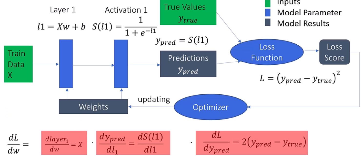
5. Bias Gradients: Similarly, we need to calculate the gradients for the biases. The steps are the same as for the weights:
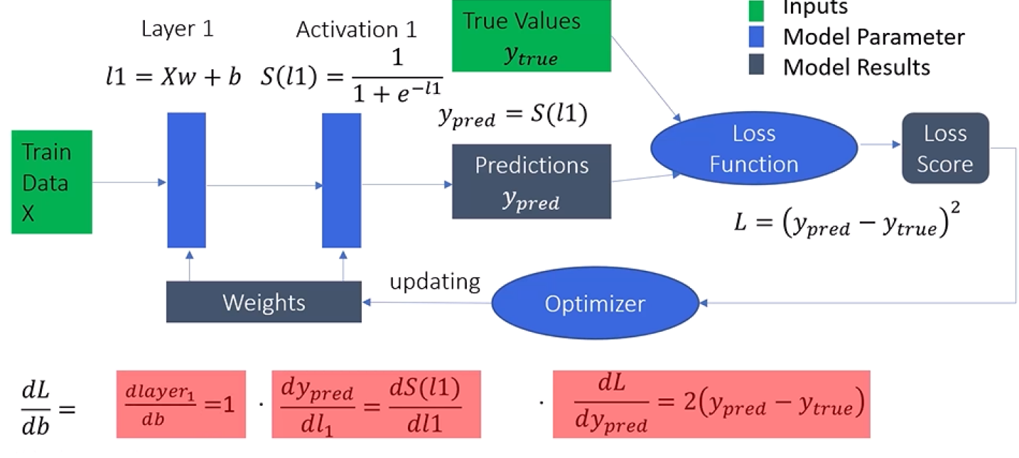
6. Update Weights and Biases: Finally, we update the weights and biases using the calculated gradients. This is typically done using an optimizer, such as stochastic gradient descent (SGD). The weights and biases are adjusted in the direction that reduces the loss:
w(new)=w(old)−η×dL/dwb(new)=b(old)−η×dL/dw
Here, η is the learning rate, a hyperparameter that controls the step size of the updates.
The backward pass is all about propagating the error backward through the network, calculating gradients at each step, and updating the weights and biases to minimize the loss. By doing this iteratively, we train the neural network to make better predictions.
Understanding the DOT PRODUCT
There is one more important concept we need to cover in this
blog:
the dot product. It is a key idea used in neural
networks to help map input data to output predictions by
adapting the weights.
Imagine you have some input data X and two different sets of weights. The question
is:
which set of weights is more similar to the input X? This is where the dot product
comes
in handy.
What is the Dot Product?
The dot product is a way to multiply two vectors (like our input data and weights) to see how similar they are. It is a simple calculation where we multiply corresponding elements of the vectors and then add those products together.
Why Use the Dot Product?
In neural networks, the dot product helps us determine which set
of
weights is better at mapping our input data to the desired output. By comparing the
dot
products of different weight vectors with the input X, we can see which weights are
more
similar to the input.
The weights that produce a higher dot product are more aligned with the input data,
meaning they are more likely to be correct. During training, we adjust the weights
to
maximize this alignment, which helps the network make more accurate
predictions.
In summary, the dot product is a useful tool for measuring the similarity between
input
data and weights. By using it, we can adapt the weights to better map the inputs to
the
outputs, improving the performance of our neural network.
Conclusion
In this blog, we have explored the foundational concepts of neural networks from scratch. We have covered the basics of how neural networks work, including forward and backward passes, and the importance of the dot product in adjusting weights to map input data to outputs. We have also discussed key concepts like gradient descent and the chain rule, which are crucial for understanding how neural networks learn and optimize.
By breaking down these core ideas, we have built a solid foundation for understanding neural networks. In our next blog, we will take these concepts further by implementing a neural network from scratch using PyTorch. This will allow us to see these principles in action and understand how to apply them in real-world scenarios.
Stay tuned for our next blog, where we dive into the PyTorch implementation of neural networks!

Written By
Impetus Ai Solutions
Impetus is a pioneer in AI and ML, specializing in developing cutting-edge solutions that drive innovation and efficiency. Our expertise extends to product engineering, warranty management, and building robust cloud infrastructures. We leverage advanced AI and ML techniques to provide state-of-the-art technological and IT-related services, ensuring our clients stay ahead in the digital era.